Excel bar and line chart together
You can also go into Excel by double-clicking your chart. You will see a new menu item displayed in the main menu that says Chart Tools.

2 Easy Ways To Make A Line Graph In Microsoft Excel Line Graph Worksheets Line Graphs Charts And Graphs
I have a chart with two axis on the X axis I have the date on the two Y axis i have bar and line data.

. It is no longer essential to rely on the manual making of the chart in Microsoft Excel as most individuals do. Types of Charts in Excel Types Of Charts In Excel Excel offers a variety of chart types based on your requirements. You now have all the data you need to put together a stacked bar chart the stepping stone to the future funnel graph.
The SUM Function Adds numbers together. Click Insert Column or Bar Chart Choose Stacked Bar Right away a simple stacked bar chart will pop up. In the chart shown in this example daily sales are plotted in columns and a line shows target sales of 500 per day.
When you return to Word click Refresh Data to update your chart to reflect any changes made to the data in Excel. Let us consider the data of the previous example again. The horizontal line may reference some target value or limit and adding the horizontal line makes it easy to see where values are above and below this reference value.
After being rotated my pie chart in Excel looks neat and well-arranged. When you want to display the sets of the same type of data but the ranges vary widely between. More than a bar chart this helps to represent data of comparison in more than one category.
Change Chart Type allows you to switch from a pie chart to a line graph and so on using the same set of data. To use the SUM Excel Worksheet Function select a cell and type. The status bar also shows you the count and the average of the selected range very useful if you just need to check a statistic quickly.
This gives you the value for plotting the base columnbar of the stacked chart. Maybe the bar chart wasnt appropriate for the panel chart. If youve already created a Pie chart and now want to convert it to a Bar of pie chart instead here are the steps you can follow.
A common task is to add a horizontal line to an Excel chart. Click anywhere on the chart. How to Create Pie Chart in Excel.
Like all the other tabs in the ribbon INSERT tab offers its own features and tools. Customize your graphs appearance. To do so click the Design tab near the top of the Excel window then click on an option in the Chart Styles group.
Create Area Chart in Excel. Is there a formula or a quick way in Excel 2003 to do this. Click the line graph and bar graph icon.
A pie chart sometimes called a circle chart is a useful tool for displaying basic statistical data in the shape of a circle each section resembles a slice of pieUnlike in bar charts or line graphs you can only display a single data series in a pie chart and you cant use zero or negative values when creating oneA negative value will display as its positive equivalent and a. Since the category axes of column and line charts work the same way lets do them together starting with the. If youre using a slightly older version of Excel the location of each feature mentioned below might be slightly different.
Example 2The 100 2D Stacked Bar Chart. Now lets move to the advanced steps of editing this chart. Click the radio button next to Secondary axixs.
When want to display two different data sets together and 2. All Excel formulas begin with the equals sign followed by a specific text tag denoting the formula youd like Excel to perform. Set up a stacked bar chart.
Comparison Charts are also known with a famous name as Multiple Column Chart or Multiple Bar Chart. This is a type of bar chart or column chart. In the Select Data Source window click the Add button.
Highlight all the chart data A1C6. The bar in the chart is actually hidden behind the clustered chart. Easily insert advanced charts.
How to Convert a Pie Chart to a Bar of Pie Chart. Rotate 3-D charts in Excel. This is a Comparison Chart in Excel.
Under Chart Tools select the Design tab. In the Insert tab Insert Tab In excel INSERT tab plays an important role in analyzing the data. Here we discuss how to create a comparison chart in Excel together with practical examples and an Excel template for download.
With the help of ready-made Excel chart templates making premium charts is an easy process saving you precious time and energyYou can find XLS samples you can incorporate into dashboards speedometers wedding seating medication pitching stocks and much more. The steps to create a 100 2-D stacked bar chart are listed as follows. The following formulas apply to the latest version of Excel.
This will change the way your graph looks including the color schemes used the text allocation and whether or not percentages are displayed. A clustered bar chart is generally known as a grouped bar chart. Thus you can see that its quite easy to rotate an Excel chart to any angle till it looks the way you need.
Your researchers could probably handle logarithmic axes which scare many. From the Insert Chart dialog box select the All Charts Bar Chart Clustered Bar Chart. First insert the named range Profit_Margin linked to the actual values column B into the chart.
I want the 70 to show a label without putting in a text box eg 70 and none of the other figures will have the sign. Combo charts combine more than one Excel chart type in the same chart. Now look at the Format tab.
A line-column chart combines a line graph and column chart on the same graph. Right-click on the empty chart and choose Select Data from the contextual menu. The ultimate Excel charting Add-in.
Its helpful for fine-tuning the layout of the labels or making the most important slices stand out. Click on the chart youve just created to activate the Chart Tools tabs on the Excel ribbon go to the Design tab Chart Design in Excel 365 and click the Select Data button. 6 Click the icon that resembles a bar chart in the menu to the right.
You can also go through our other suggested articles. Double-click the line you want to graph on a secondary axis. For our example we will create a column chart Insert Column or Bar Chart Clustered Column.
The free Chart Alignment Add-in for Excel allows you to quickly align the objects within a chart. I have a similar problem with Excel 2013. To view the Design tab your chart must be.
This is displayed as a positive result. This will insert a Simple Clustered Bar Chart. Once you decide on a graph format you can use the Design section near the top of the Excel window to select a different template change the colors used or change the graph type entirely.
I generally would have used a line chart or dot plot. Its messy with multiple series In any case if you want to look at trends you may need another chart type and just deal with the range of values. You can even select 3D Clustered Bar Chart from the list.
One way you can use a combo chart is to show actual values in columns together with a line that shows a goal or target value. Spin pie column line and bar charts. The two charts share an X axis but each has its own Y axis.
The Line data shows from 30 to 70 in increments of 10. _ Positive Variance The variance is calculated as the variance between series 1 and series 2 actual and budget. Introduction to Grouped Bar Chart.
Or click the Chart Filters button on the right of the graph and then click the Select Data link at the bottom. Right-click on the Bar representing Year 2014 and select Format. There are two common uses for a combination chart.
Where the bar chart draws the relation of two parameters this can consider the higher version of the bar chart. Excel 2003 allowed me to glue 2 or more charts together using GROUP command. Column Charts Line Charts Pie Charts Bar Charts Area Charts Scatter Charts Stock Chart and Radar Charts are the different types of charts.
Then I can copy or cut the whole thing that includes all the GROUPED charts to somewhere else. Add the named rangeranges containing the actual values. Customize your charts appearance.
This example uses a combo chart based on a column chart to plot. Go to the Insert tab.

Excel How To Create A Dual Axis Chart With Overlapping Bars And A Line Chart Visualisation Excel

How To Plot Combined Line And Bar Chart Of Two Measurements In Excel Bar Chart Chart Excel

Excel Variance Charts Making Awesome Actual Vs Target Or Budget Graphs How To Pakaccountants Com Excel Shortcuts Excel Tutorials Excel Hacks

Conditional Formatting Intersect Area Of Line Charts Line Chart Chart Intersecting
How To Add A Secondary Axis In Excel Charts Easy Guide Trump Excel Excel Chart Chart Tool

Create Line Charts With Confidence Bands Line Chart Chart Tool Chart

Highlight A Time Period On A Line Chart Chart Line Chart Period

Graphs And Charts Vertical Bar Chart Column Chart Serial Line Chart Line Graph Scatter Plot Ring Chart Donut Chart Pie Chart Dashboard Design Bar Chart

Side By Side Bar Chart Combined With Line Chart Welcome To Vizartpandey Bar Chart Chart Line Chart

Microsoft Excel Dashboard Excel Tutorials Microsoft Excel Microsoft Excel Tutorial

Adding Up Down Bars To A Line Chart Chart Excel Bar Chart

Bar Chart Inspiration Buscar Con Google Bar Chart Chart Excel

Multiple Width Overlapping Column Chart Peltier Tech Blog Data Visualization Chart Multiple

Try Using A Line Chart In Microsoft Excel To Visualize Trends In Your Data Line Chart Excel Microsoft Excel Tutorial
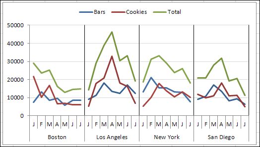
How To Create A Panel Chart In Excel Chart Excel Shortcuts Excel

Charts In Excel Excel Tutorials Chart Excel Templates

Excel How To Create A Dual Axis Chart With Overlapping Bars And A Line Excel Excel Tutorials Circle Graph